Machine Learning

WORK IN PROGRESS

The fundamentals of Machine Learning using Python

What is machine learning?

AI vs MACHINE LEARNING vs DEEP LEARNING

Artificial intelligence (AI) is the science that empowers computers to mimic human intelligence or behavior such as decision making, text processing and visual perception. One subfield of AI is Machine Learning (ML) that enables machines to improve at a given task with experience. Other subfields of ML include robotics or computer vision. Machine Learning has also various subfields: Supervised Learning, Unsupervised Learning and Reinforcement Learning. Deep Learning (DL) is a specialized field of Machine Learning that relies on training of Deep Artificial Neural Networks (ANN), which are inspired by the human brain, using a large dataset such as images or texts.

SUPERVISED LEARNING

Supervised Learning algorithms are trained algorithms using labeled input/output data

Regression

Regression models (both linear and non-linear) are used for predicting a continuous real value, like salary for example. Regression technique vary from Linear Regression to SVR and Random Forests Regression.

1. Simple Linear Regression
2. Multiple Linear Regression
3. Polynomial Regression
4. Support Vector for Regression (SVR)
5. Decision Tree Classification
6. Random Forest Classification

1. Simple Linear Regression

Simple linear regression is used to determine the relationship between two variables. That is, given one independent variable x, it tells us what we can expect from the dependent variable y. y = alpha + beta * x

Example

2. Multiple Linear Regression

Multiple linear regression attempts to model the relationship between two or more explanatory variables and a response variable by fitting a linear equation to observed data. Every value of the independent variable x is associated with a value of the dependent variable y.

• Pros: Works on any size of dataset, gives informations about relevance of features
• Cons: The Linear Regression Assumptions
  • A Linear Relationship between the outcome variable and the independent variables. A plot of the standardized residuals verses the predicted Y’ values show whether there is a linear or curvilinear relationship.
  • Multivariate Normality – Multiple regression assumes that the variables are normally distributed.
  • No Multicollinearity – This assumption assumes that the independent variables are not highly correlated with each other. This assumption is tested by the Variance Inflation Factor (VIF) statistic.
  • Homoscedasticity – This assumption requires that the variance of error terms are similar across the independent variables. As with the linear relationship assumption, Intellectus Statistics plot the standardized residuals verses the predicted Y’ values can show whether points are equally distributed across all values of the independent variables or not.

Example

Classification

In classification you predict a category or a class.

UNSUPERVISED LEARNING

Unsupervised Learning algorithms are trained algorithms with no labeled data. It attempts at discovering hidden patterns on its own.

Clustering

REINFORCEMENT LEARNING

Algorithms take actions to maximize cumulative reward.

Data preprocessing

Data was preprocessed as follows:

# Import the libraries
import numpy as np
import matplotlib.pyplot as plt
import pandas as pd

# Import dataset
dataset = pd.read_csv('Data.csv')
X = dataset.iloc[:, :-1].values
y = dataset.iloc[;.-1].values
    
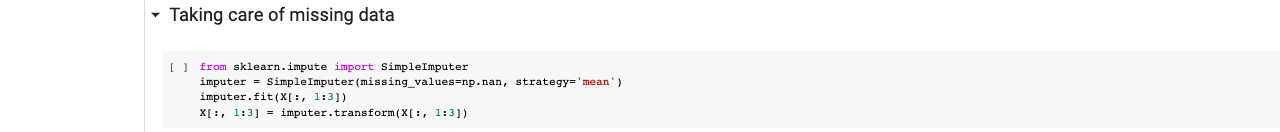
# Take care of missing data using imputation
from sklearn.impute import SimpleImputer
imputer = SimpleImputer(missing_values = np.nan, strategy = 'mean')
imputer.fit(X[:, 1:3])
X[:, 1:3] = imputer.transform(X[:,1:3]) 

# Encoding categorical data
from sklearn.compose import ColumnTransformer
from sklearn.preprocessing import OneHotEncoder
ct = ColumnTransformer(transformers=[('encoder','OneHotEncoder'(),[0])], remainder='passthrough' 
X = np.array(ct.fit_transform(X))

from sklearn.preprocessing import LabelEncoder
le = LabelEncoder()
y = le.fit_transform(y)

For training the machine learning algorithms the dataset was split into a training ((80%) and test set (20%):

from sklearn.model_selection import train_test_split
X_train, X_test, y_train, y_test = train_test_split(X, y, test_size = 0.2, random_state = 1)

For some of the machine learning models feature scaling was applied in order to avoid that some features are dominated by other features and are not considered by the model.

Feature scaling is a technique that will get the mean and standard deviation and apply two techniques:

1. Standardisation: subtracting each value of a specific feature by the mean of all the values of this feature and then dividing by the standard deviation (which is the square root of the variance). This will put all the values of the feature between around minus three and plus three.
2. Normalisation: subtracting each value of a specific feauture by the minimum value of this feature and then dividing by the difference between the maximum value and the minimum value of this feature. All the values of the features will become between 0 and 1.

Standardization actually works well all the time, but Normalization is recommended when there is a normal distribution in most of the features.

Feature scaling needs to be applied after the data split, as the test set is supposed to be a brand new data set that the model has never seen before. If we were to include the test data in the feature scaling process, the test data would be incorporated in the training set as well and cause information leakage.

Dummy variables do not need to be standardised as they are already within the range of -3 and 3 and it will make interpretation more difficult.

from sklearn.preprocessing import StandardScaler
sc = StandardScaler()
X_train[:,3:] = sc.fit_transform(X_train[:,3:])
X_test[:,3:] = sc.transform(X_test[:,3:])